beer_markets <- read_csv("https://bcdanl.github.io/data/beer_markets_all.csv")Analyzing Market Dynamics and Consumer Behavior in the Beer Industry
Data-Driven Mastery: Unlocking Business Potential
1 Beer Market Data
1.1 Variable Description
‘hh’: an identifier of the household
‘X_purchase_desc’: details on the purchased item
‘quantity’: the number of items purchased
‘brand’: Bud Light, Busch Light, Coors Light, Miller Lite, or Natural Light
‘dollar_spent’: total dollar value of purchase
‘beer_floz’: total volume of beer, in fluid ounces
‘price_per_floz’: price per fl.oz. (i.e., beer spent/beer floz)
‘container’: the type of container
‘promo’: Whether the item was promoted (coupon or otherwise)
‘market’: Scan-track market (or state if rural)
‘state’: US State
demographic data, including gender, marital status, household income, class of work, race, education, age, the size of household, and whether or not the household has a microwave or dishwasher
2 Introduction
2.1 Background
The beer industry is one of the largest sectors of the global beverage market. Beer is a staple for millions of people whether it be for a celebration, social gathering, of just everyday life. Like everything in the world, the beer market is constantly evolving due to trends in the market and consumer preference changes. One consumer preference in the beer market is light beer and almost every beer company makes their own light beer. The beer markets data includes data about Bud Light, Busch Light, Coors Light, Miller Lite, and Natural Light. I am going to analyze the beer markets data to find information about brand preferences, purchasing patterns, and beer consumption trends. This information is significant because it can provide insight into competitive challenges, market opportunities, and areas of innovation and growth for breweries and retailers.
2.2 Statement of the Problem
The overall goal of breweries and retailers that sell beer is to maximize profits. In order to do this, they need to understand factors that drive consumer behavior and influence their purchasing decisions. They also need to find their specific target market and cater their beer to meet the needs of this target market. Factors in the target market include income, employment, age, race, housing, and family dynamic. I am going to analyze the dynamics and consumer behavior in the beer markets data. In doing so, I will gain an understanding of beer consumption trends, brand preferences, and purchasing patterns. I will see what the target market for each brand is and also see information about their promotions to see how this effects purchasing patterns. The problem this will address is decision making for breweries and retailers. The insight provided from the analysis of this data will tell them about competitive challenges, market opportunities, potential changes, and areas of innovation or growth to help guide their decision making in order to maximize profits.
3 Exploratory Data Analysis
3.1 Question 1
- What is the most popular beer brand purchased at each income level?
- Does income have an impact on which brand consumers purchase?
Answer:
beer_markets |>
  distinct(income)
# A tibble: 5 × 1
income
<chr>
1 20-60k
2 100-200k
3 60-100k
4 under20k
5 200k+ beer_markets2 <- beer_markets %>%
mutate(income_numeric = case_when(
income == "under20k" ~ 20000,
income == "20-60k" ~ 60000,
income == "60-100k" ~ 100000,
income == "100-200k" ~ 200000,
income == "200k+" ~ 500000))beer_brand_purchases <- beer_markets2 |>
group_by(income, income_numeric, brand) |>
summarize(total_quantity = sum(quantity))
most_popular_brands_by_income <- beer_brand_purchases |>
group_by(income, income_numeric) |>
filter(total_quantity == max(total_quantity)) |>
select(income, income_numeric, brand, total_quantity)
brand_distribution <- beer_brand_purchases |>
group_by(income, income_numeric) |>
mutate(percentage = total_quantity / sum(total_quantity) * 100) |>
arrange(desc(income_numeric))Bud Light is the most purchased brand at every income level besides the 60-100K level where Miller Lite is the most popular. Income does not appear to have an impact on which brand consumers purchase since Bud light is the most popular for the lowest and highest income level.
ggplot(brand_distribution, aes(x = income_numeric, y = percentage, fill = brand)) +
  geom_bar(stat = "identity", position = "stack") +
  labs(title = "Most Commonly Purchased Brands Based On Income",
       x = "Income",
       y = "Percentage") +
  scale_x_continuous(
    breaks = unique(brand_distribution$income_numeric),
    labels = unique(brand_distribution$income)) +
  theme_minimal() +
  theme(axis.text.x = element_text(angle = 45, hjust = 1))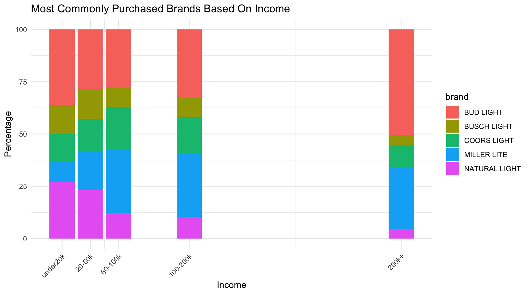
The most obvious trends visible from this is that as income increases, the percentage of Natural Light and Busch Light decrease. As Natural Light and Busch Light are decreasing, Miller Lite and Bud Light are both increasing in percentage as income increases. This indicated that Natural Light and Busch Light are more popular with lower income customers and Miller Lite and Bud Light are more popular with higher income customers.
3.2 Question 2
- Which income level buys the most beer?
Answer:
beer_quantity <- beer_markets2 |>
  group_by(income, income_numeric) |>
  summarise(total_quantity = sum(quantity, na.rm = TRUE)) |>
  arrange(desc(total_quantity))

ggplot(beer_quantity,
       aes(x = income_numeric, y = total_quantity)) +
  geom_point() +
  geom_line() +
  labs(title = "Quantity of Beer Purchased Based On Income",
       x = "Income",
       y = "Total Quantity") +
  scale_x_continuous(breaks = beer_quantity$income_numeric,
                     labels = beer_quantity$income) +
  theme_minimal() +
  theme(axis.text.x = element_text(angle = 45, hjust = 1))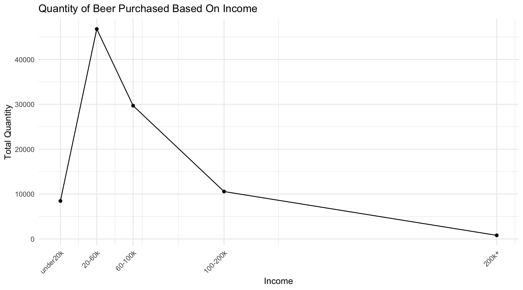
The income level that purchases the most beer is 20-60k at 46,786. As income level increases, the quantity of beer purchased exponentially decreases as it goes all the way down to 812 for those making 200k+. People making under 20k were the second least with 8,469 most likely due to their limited budget.
3.3 Question 3
- Does income have an impact on the dollars spent on a purchase?
Answer:
spent_per_income <- beer_markets2 |>
  group_by(income, income_numeric) |>
  summarize(avg_dollar_spent = mean(dollar_spent, na.rm = TRUE)) |>
  arrange(desc(income_numeric))

rmarkdown::paged_table(spent_per_income)
Income does have a direct impact on the average amount of money that a customer spends on beer. As income increases, so does the average dollar amount that they spent. For those making under 20k, they spent an average of 13.51 dollars while those making 200k+ spent an average of 15.12 dollars. This makes sense because the customers with higher income have more money to spend.
3.4 Question 4
- What percentage of purchases in each income level are made during a promotion?
Answer:
beer_promotion <- beer_markets2 |>
  select(income, income_numeric, promo)

promo_percentage <- beer_promotion |>
  group_by(income, income_numeric) |>
  summarize(promo_percent = mean(promo) * 100)

ggplot(promo_percentage,
       aes(x = income_numeric, y = promo_percent)) +
  geom_point() +
  geom_line() +
  labs(title = "Promotion Purchases Based On Income",
       x = "Income",
       y = "Percentage") +
  scale_x_continuous(breaks = promo_percentage$income_numeric,
                     labels = promo_percentage$income) +
  theme_minimal() +
  theme(axis.text.x = element_text(angle = 45, hjust = 1))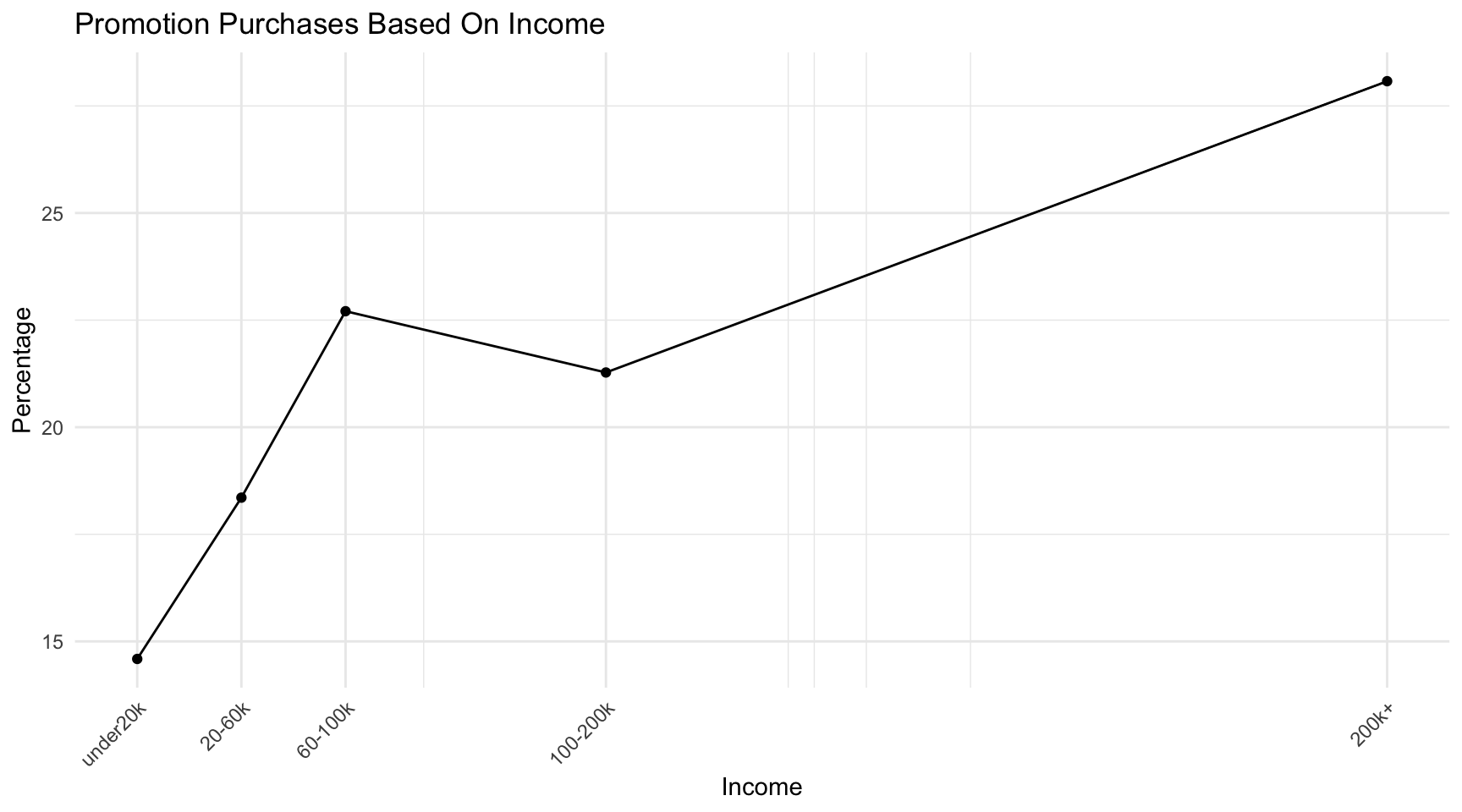
There is almost a direct correlation between income and percentage of purchases made during a promotion. The correlation is that as income increases, so does the percentage of purchases made during a promotion. This is true for all values other than a slight decrease from the 60-100k to the 100-200k income levels. This shows that people with a higher income are usually more likely ot respond to a promotion for beer.
3.5 Question 5
- Which states buy the most beer overall?
- Which state buys the most of each brand?
Answer:
brand_by_state <- beer_markets |>
  group_by(state, brand) |>
  summarize(total_quantity = sum(quantity))

most_popular_brand_by_state <- brand_by_state |>
  group_by(state) |>
  filter(total_quantity == max(total_quantity)) |>
  select(state, brand, total_quantity) |>
  arrange(desc(total_quantity))

top_states_for_each_brand <- brand_by_state |>
  group_by(brand) |>
  arrange(desc(total_quantity)) |>
  group_by(brand) |>
  slice_head(n = 2)

beer_quantity_by_state <- beer_markets |>
  group_by(state) |>
  summarize(total_quantity = sum(quantity)) |>
  arrange(desc(total_quantity))

most_popular_state_for_brand <- brand_by_state |>
  group_by(brand) |>
filter(total_quantity == max(total_quantity))ggplot(beer_quantity_by_state, aes(x = state, y = total_quantity)) +
geom_bar(stat = "identity", width = 0.7) +
labs(title = "Total Quantity of Beers Purchased by State",
x = "State",
y = "Total Quantity") +
theme_minimal() +
theme(axis.text.x = element_text(angle = 90, hjust = 1))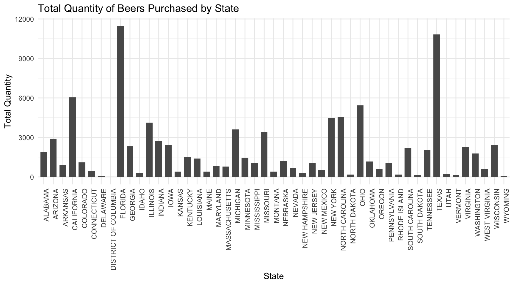
This data can help the brands determine where they need to distribute the most stock and which state they should target the most. For example, Florida and Texas have by far more beer sales than the rest of the states, so they will require a larger stock.
ggplot(top_states_for_each_brand, aes(x = brand, y = total_quantity, fill = state)) +
  geom_bar(stat = "identity", position = "dodge") +
  labs(title = "Top States for Each Brand",
       x = "Brand",
       y = "Total Quantity",
       fill = "State") +
  theme_minimal() +
  theme(axis.text.x = element_text(angle = 45, hjust = 1))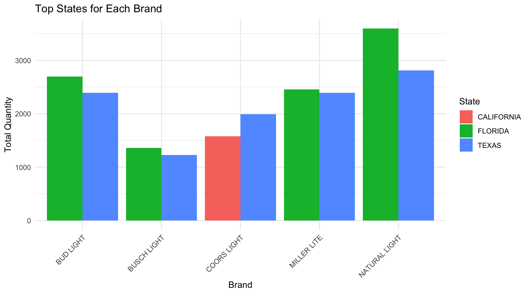
Natural Light in Florida is the highest total quantity out of all beers in every state. This will help retailers in Florida know that they need to order a lot of Natural Light to always keep it in stock since there is such high demand. California shows up only one time and it is for Coors Light so that will help retailers in California know they need to order a good amount of Coors Light. Overall every brand is going to need to send a large quantity of their beer to Texas because that is the state with either the most or second most purchased of each brand.
3.6 Question 6
- Which age group purchases the most beer?
- What are the most popular brands for each age group?
Answer:
beer_markets |>
  distinct(age)
# A tibble: 4 × 1
age
<chr>
1 50+
2 40-49
3 30-39
4 <30 beer_markets2 <- beer_markets2 |>
mutate(age_numeric = case_when(
age == "<30" ~ 25,
age == "30-39" ~ 35,
age == "40-49" ~ 45,
age == "50+" ~ 55))beer_by_age <- beer_markets2 |>
group_by(age, age_numeric) |>
summarize(total_quantity = sum(quantity, na.rm = TRUE)) |>
arrange(desc(total_quantity))
ggplot(beer_by_age,
aes(x = age, y = total_quantity, color = age, size = 2)) +
geom_point() +
labs(title = "Beers Purchased By Age",
x = "Age",
y = "Quantity") +
theme_minimal()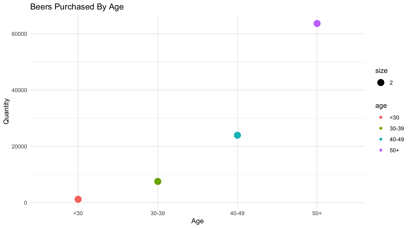
The quantity of beer purchased exponentially increases as age increases. This can help the beer companies and retailers, because knowing that 50+ is their largest customer, they can target advertisements to appeal to them.
brand_by_age <- beer_markets2 |>
  group_by(age, age_numeric, brand) |>
  summarize(total_quantity = sum(quantity, na.rm = TRUE)) |>
  arrange(age_numeric, desc(total_quantity))

ggplot(brand_by_age,
       aes(x = age_numeric, y = total_quantity, color = brand)) +
  geom_point() +
  geom_line() +
  labs(title = "Most Popular Brands For Each Age",
       x = "Age",
       y = "Quantity") +
  scale_x_continuous(breaks = brand_by_age$age_numeric,
                     labels = brand_by_age$age) +
  theme_minimal()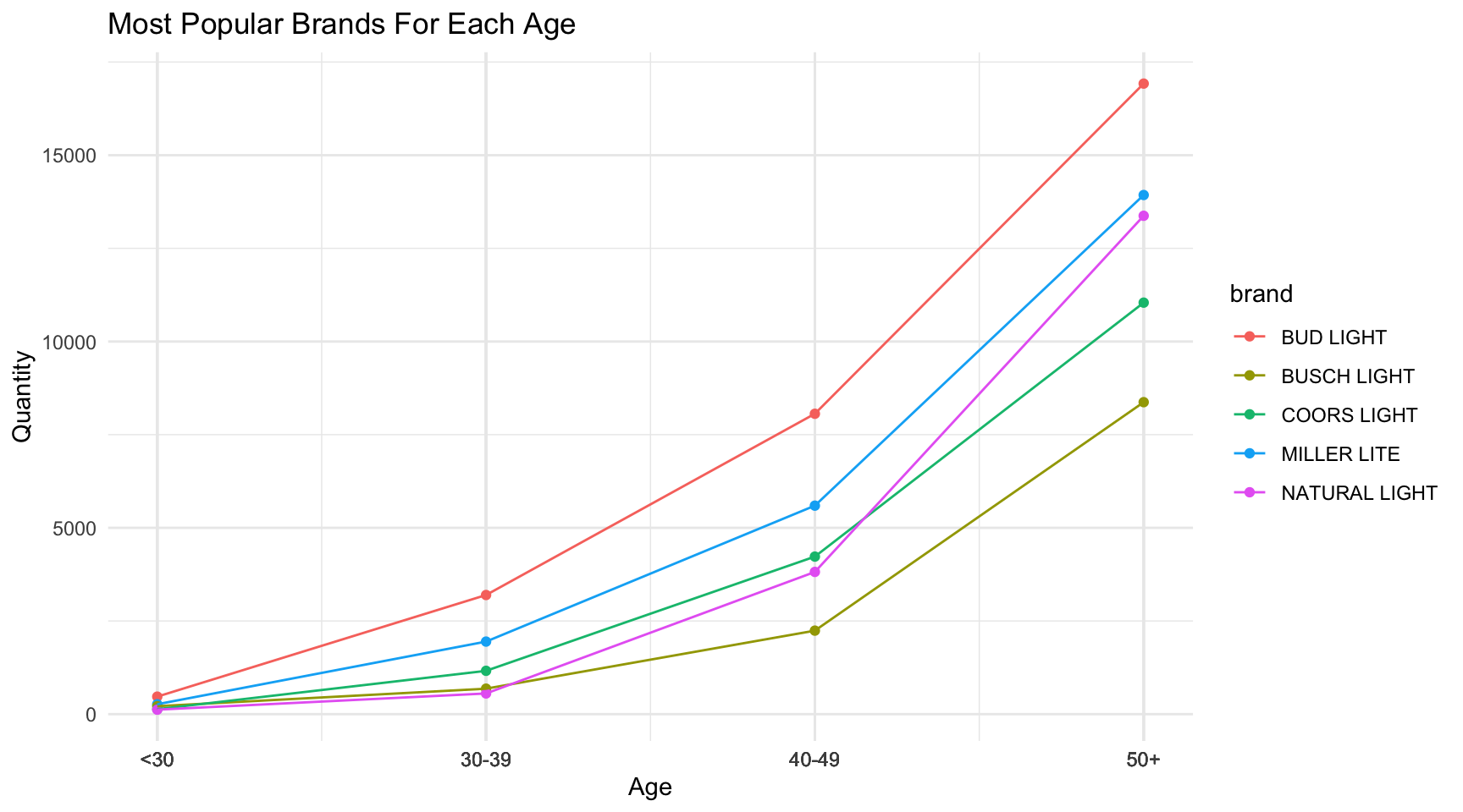
Bud Light is the most popular brand and Miller Lite is the second most popular brand for every age group. Busch Light is the least popular for every age group. The difference between Bud Light and Busch Light gets larger as age increases. This information can be helpful to retailers because it will help them determine how many of each brand to have in stock depending on the typical age of their customer.
3.7 Question 7
- What is the distribution of each beer brand purchased by buyer type?
Answer:
buyer_type_purchases <- beer_markets2 |>
  group_by(buyertype, brand) |>
  summarize(count = n()) |>
  arrange(buyertype, desc(count))

ggplot(beer_markets2,
       aes(x = buyertype, fill = brand)) +
  geom_bar(position = "dodge") +
  labs(title = "Distribution of Beer Brands by Buyer Type",
       x = "Buyer Type",
       y = "Count") +
  theme_minimal()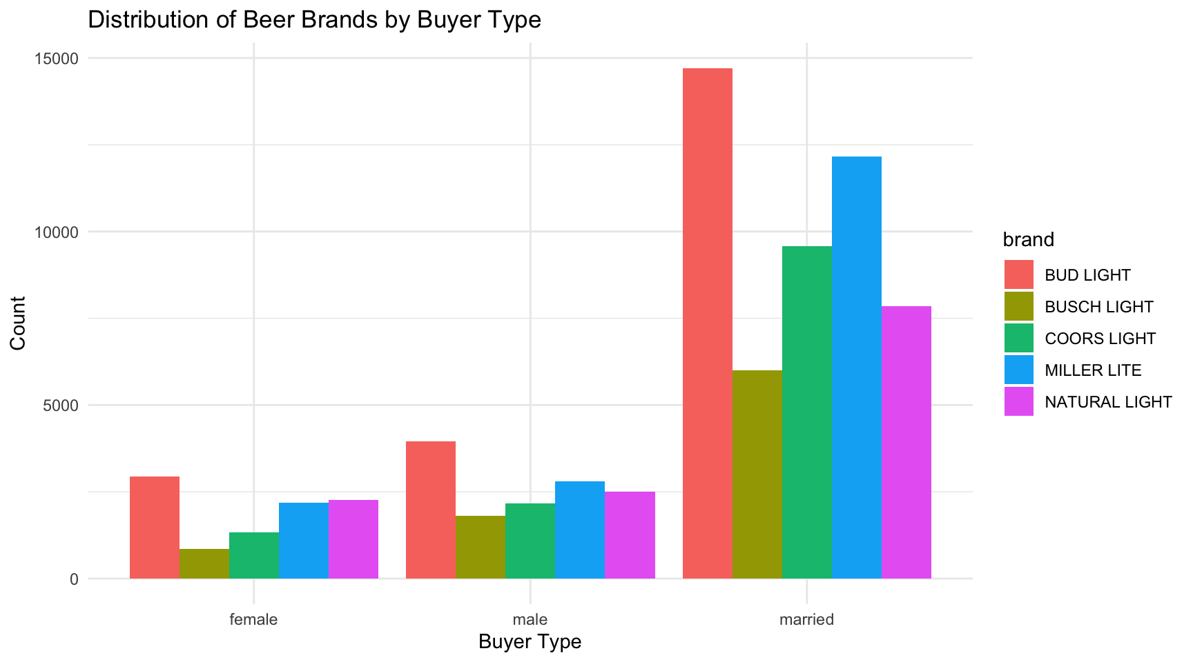
Buyers who are married buy significantly more beer than individual male or female buyers. Males buy a little bit more than females for every brand. Bud Light is the most frequently purchased by every buyer type with 14,706 in the married type being the most in the data.. Busch Light is the lowest for each group with only 864 purchased by females being the least in the data.
3.8 Question 8
- What is the total number of beers purchased by each race?
- Is there a significant brand preference for any race?
Answer:
race_beer_total <- beer_markets2 |>
  group_by(race) |>
  summarize(total_beers = sum(quantity, na.rm = TRUE)) |>
  arrange(desc(total_beers))

race_brand_totals <- beer_markets2 |>
  group_by(race, brand) |>
  summarize(total_quantity = sum(quantity)) |>
  ungroup()

race_brand_percentage <- race_brand_totals |>
  left_join(race_beer_total, by = "race") |>
mutate(percentage = (total_quantity / total_beers) * 100)ggplot(race_brand_percentage,
aes(x = race, y = percentage, fill = brand)) +
geom_bar(stat = "identity", position = "stack") +
labs(title = "Percentage of Beer Brand Purchases by Race",
x = "Race",
y = "Percentage") +
theme_minimal()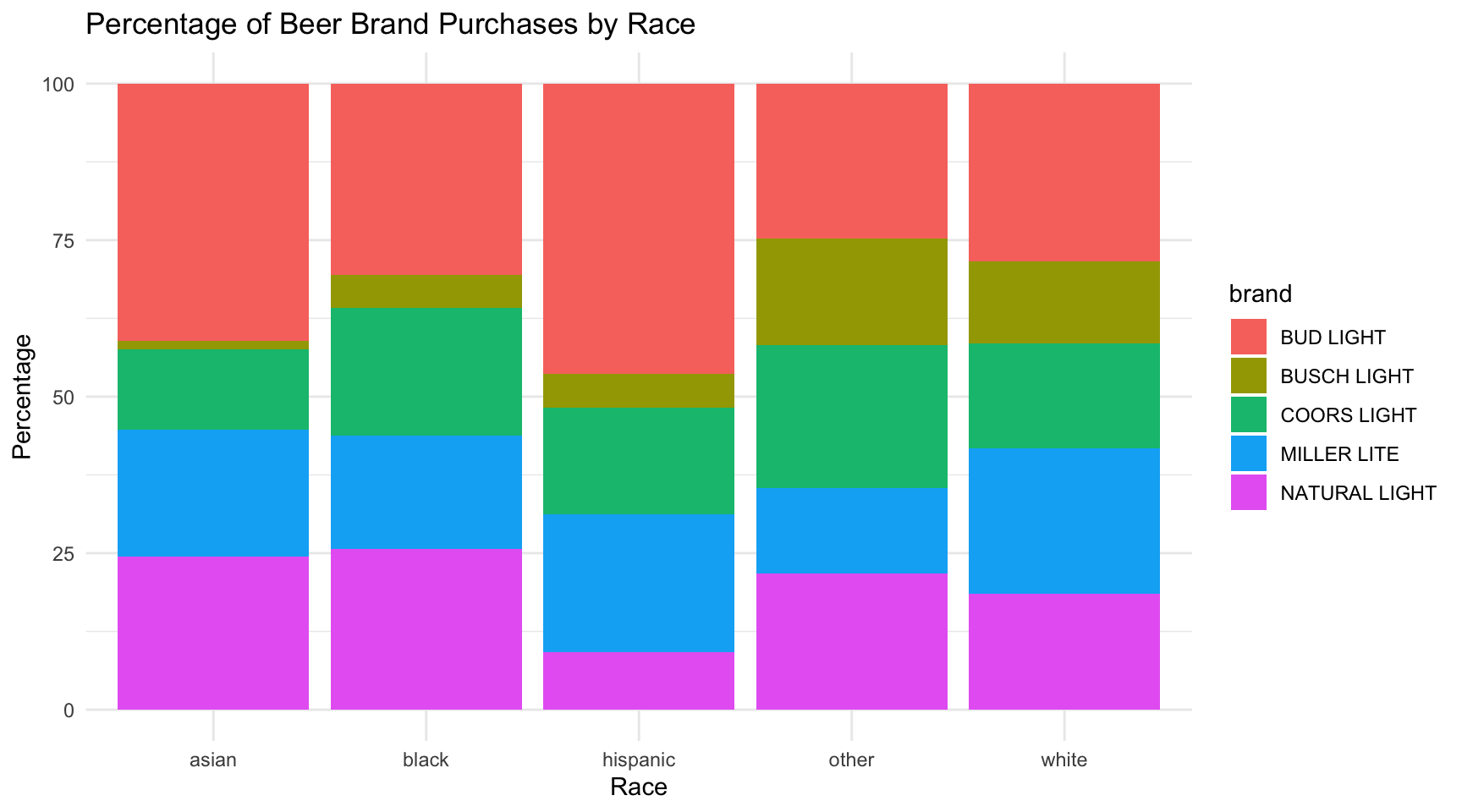
ggplot(race_brand_percentage,
       aes(x = race, y = percentage, fill = brand)) +
  geom_bar(stat = "identity", position = "dodge") +
  labs(title = "Percentage of Beer Brand Purchases by Race",
       x = "Race",
       y = "Percentage") +
  theme_minimal()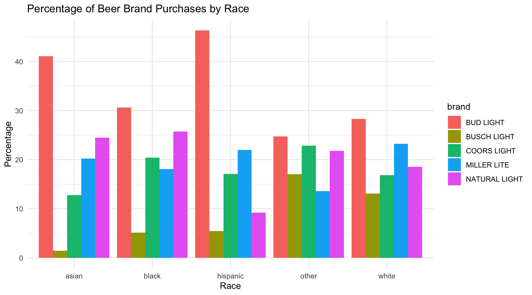
Bud Light is most frequently purchased brand for every race in this data. Hispanic and Asian customers purchase Bud Light over 40 percent of the time that they are purchasing beer with Hispanics all the way at 46.34 percent. Asian customers purchasing Busch Light is by far the lowest percentage with it making up only 1.42 percent of their beer purchases.
3.9 Question 9
- Which employment types purchase the most beer?
- What is the quantity of each beer brand for each employment type?
Answer:
employment_beers <- beer_markets2 |>
  group_by(employment) |>
  summarize(total_quantity = sum(quantity, na.rm = TRUE)) |>
  arrange(desc(total_quantity))

rmarkdown::paged_table(employment_beers)
employment_brands <- beer_markets2 |>
group_by(employment, brand) |>
summarize(total_quantity = sum(quantity, na.rm = TRUE)) |>
arrange(desc(total_quantity))
ggplot(employment_brands,
aes(x = employment, y = total_quantity, fill = brand)) +
geom_col(position = "dodge") +
labs(title = "Quantity of Beer Brands by Employment Status",
x = "Employment Status",
y = "Quantity") +
theme_minimal()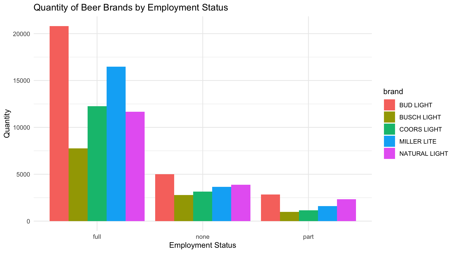
Customers with full time employment purchased significantly more beers than customers with part time of no employment. Full time purchased 68,939, while unemployed purchased 18,456, and part time purchased only 8,936. Bud Light was the most purchased brand for each employment type but was significantly more for those with full time employment at 20,810.
3.10 Question 10
- Which degree types purchase the most beer?
- What is the quantity of each beer brand for each degree?
Answer:
degree_totals <- beer_markets2 |>
  group_by(degree) |>
  summarize(total_quantity = sum(quantity)) |>
  arrange(desc(total_quantity))

rmarkdown::paged_table(degree_totals)
degree_brands <- beer_markets2 |>
group_by(degree, brand) |>
summarize(total_quantity = sum(quantity, na.rm = TRUE)) |>
arrange(desc(total_quantity))
ggplot(degree_brands,
aes(x = degree, y = total_quantity, fill = brand)) +
geom_col(position = "dodge") +
labs(title = "Quantity of Beer Brands by Degree",
x = "Degree",
y = "Quantity") +
theme_minimal()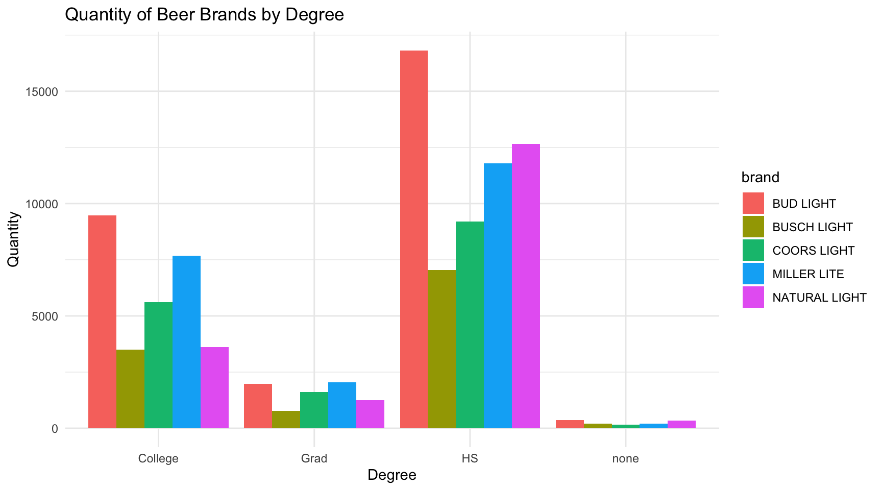
Customers with a HS degree purchase the most beer followed by those with college degrees. Bud Light is the most purchased by every degree type with 16,816 for HS degree customers. Natural Light is the second highest for HS degree and customers with no degree while Miller Lite is the second highest for college and grad degree customers.
3.11 Question 11
- What is the most common combination of income, state, age, buyertype, race, employment, and degree that purchased the largest quantity of each beer brand?
- What are the ten most common combinations of income, state, age, buyertype, race, employment, and degree that purchased the largest quantity of each beer brand?
Answer:
target_market <- beer_markets2 |>
  group_by(brand, income, state, age, buyertype, race, employment, degree) |>
  summarize(total_quantity = sum(quantity)) |>
  ungroup()

brand_most_purchased <- target_market |>
  group_by(brand) |>
  arrange(desc(total_quantity)) |>
  slice_head(n = 1)

rmarkdown::paged_table(brand_most_purchased)
This shows the specific income, state, age, buyertype, race, employment, and degree combination that purchased the most of each beer brand. The most purchased brand by one of these specific combinations is Bud Light with 1,080 total. These customers had an income under 20k, live in New York, are between 40-49 years old, female, Hispanic, have part time employment, and a college degree. This breakdown can help the beer brands find out what target market they are selling the most to and meet the needs of these specific customers.
brand_target_market <- target_market |>
  group_by(brand) |>
  arrange(desc(total_quantity)) |>
  slice_head(n = 10)

rmarkdown::paged_table(brand_target_market)
This shows the 10 most common specific combinations of income, state, age, buyertype, race, employment, and degree that purchased each beer brand. This data will further help the beer brands understand their target market and meet their needs.
4 Significance of the Project
4.1 Question 1
Bud Light is the most purchased brand at every income level besides the 60-100K level where Miller Lite is the most popular. Income does not appear to have an impact on which brand consumers purchase since Bud light is the most popular for the lowest and highest income level.
The most obvious trends visible from this is that as income increases, the percentage of Natural Light and Busch Light decrease. As Natural Light and Busch Light are decreasing, Miller Lite and Bud Light are both increasing in percentage as income increases. This indicated that Natural Light and Busch Light are more popular with lower income customers and Miller Lite and Bud Light are more popular with higher income customers.
4.2 Question 2
The income level that purchases the most beer is 20-60k at 46,786. As income level increases, the quantity of beer purchased exponentially decreases as it goes all the way down to 812 for those making 200k+. People making under 20k were the second least with 8,469 most likely due to their limited budget.
4.3 Question 3
Income does have a direct impact on the average amount of money that a customer spends on beer. As income increases, so does the average dollar amount that they spent. For those making under 20k, they spent an average of 13.51 dollars while those making 200k+ spent an average of 15.12 dollars. This makes sense because the customers with higher income have more money to spend.
4.4 Question 4
There is almost a direct correlation between income and percentage of purchases made during a promotion. The correlation is that as income increases, so does the percentage of purchases made during a promotion. This is true for all values other than a slight decrease from the 60-100k to the 100-200k income levels. This shows that people with a higher income are usually more likely ot respond to a promotion for beer.
4.5 Question 5
This data can help the brands determine where they need to distribute the most stock and which state they should target the most. For example, Florida and Texas have by far more beer sales than the rest of the states, so they will require a larger stock.
Natural Light in Florida is the highest total quantity out of all beers in every state. This will help retailers in Florida know that they need to order a lot of Natural Light to always keep it in stock since there is such high demand. California shows up only one time and it is for Coors Light so that will help retailers in California know they need to order a good amount of Coors Light. Overall every brand is going to need to send a large quantity of their beer to Texas because that is the state with either the most or second most purchased of each brand.
4.6 Question 6
The quantity of beer purchased exponentially increases as age increases. This can help the beer companies and retailers, because knowing that 50+ is their largest customer, they can target advertisements to appeal to them.
Bud Light is the most popular brand and Miller Lite is the second most popular brand for every age group. Busch Light is the least popular for every age group. The difference between Bud Light and Busch Light gets larger as age increases. This information can be helpful to retailers because it will help them determine how many of each brand to have in stock depending on the typical age of their customer.
4.7 Question 7
Buyers who are married buy significantly more beer than individual male or female buyers. Males buy a little bit more than females for every brand. Bud Light is the most frequently purchased by every buyer type with 14,706 in the married type being the most in the data.. Busch Light is the lowest for each group with only 864 purchased by females being the least in the data.
4.8 Question 8
Bud Light is most frequently purchased brand for every race in this data. Hispanic and Asian customers purchase Bud Light over 40 percent of the time that they are purchasing beer with Hispanics all the way at 46.34 percent. Asian customers purchasing Busch Light is by far the lowest percentage with it making up only 1.42 percent of their beer purchases.
4.9 Question 9
Customers with full time employment purchased significantly more beers than customers with part time of no employment. Full time purchased 68,939, while unemployed purchased 18,456, and part time purchased only 8,936. Bud Light was the most purchased brand for each employment type but was significantly more for those with full time employment at 20,810.
4.10 Question 10
Customers with a HS degree purchase the most beer followed by those with college degrees. Bud Light is the most purchased by every degree type with 16,816 for HS degree customers. Natural Light is the second highest for HS degree and customers with no degree while Miller Lite is the second highest for college and grad degree customers.
4.11 Question 11
This shows the specific income, state, age, buyertype, race, employment, and degree combination that purchased the most of each beer brand. The most purchased brand by one of these specific combinations is Bud Light with 1080 total. These customers had an income under 20k, live in New York, are between 40-49 years old, female, Hispanic, have part time employment, and a college degree. This breakdown can help the beer brands find out what target market they are selling the most to and meet the needs of these specific customers.
This shows the 10 most common specific combinations of income, state, age, buyertype, race, employment, and degree that purchased each beer brand. This data will further help the beer brands understand their target market and meet their needs.
4.12 Overall Significance
By using this data, beer brands and retailers can have a better understanding of their target market. This can tell them about competitive challenges, market opportunities, potential changes, and areas of innovation or growth to help guide their decision making in order to maximize profits.